Convolutional network without multiplication operation
March 14, 2019In September 2018, Google Research team released paper with the title “No Multiplication? No floating point? No problem? Training networks for efficient inference” [1] which we will refer to as NMNF. The main building blocks of convolutional neural networks are convolutional layers and the great majority of inference time is spent in them [2]. NMNF paper targets devices like hearing aids, earbuds or wearables. Such devices are highly resource constrained, in terms of memory, power, and computation, and therefore benefit from a specialized implementation of convolutional layer introduced in the paper. Inference-time floating point operations are not only energy-hungry compared to integer operations (see Table 1) but also computationally demanding. NMNF approach avoids floating point operations entirely and consequently, we can enjoy reduced model size as well.
| integer | 500 MHz | 1,200 MHz | floating point | 500 MHz | 1,200 MHz |
|---|---|---|---|---|---|
| add | 63 pJ | 105 pJ | fadd | 157 pJ | 258 pJ |
| sub | 64 pJ | 105 pJ | fsub | 158 pJ | 259 pJ |
| mul | 116 pJ | 189 pJ | fmul | 161 pJ | 265 pJ |
| div | 178 pJ | 286 pJ | fdiv | 566 pJ | 903 pJ |
Table 1: Integer and floating point arithmetic instructions with RAW dependencies measured on Cortex-A7 with frequencies 500 and 1,200 MHz. [3]
Mobile deep learning is a subfield of machine learning that focuses on optimizing and deploying deep learning models on mobile devices (mobile phones, IoT, edge devices and others). In this blog post, we describe the main characteristics of the NMNF approach and test if we can exploit the proposed solution in mobile phones. A lot of mobile deep learning applications require low latency, therefore, we will evaluate NMNF in terms of speed.
Training networks for efficient inference
The main idea behind NMNF is to precompute all possible products of input feature map with convolutional weights and store them in the lookup table (LUT). Later, during inference, instead of performing the convolution using multiplication operations, the lookup table is searched to obtain corresponding product results.
In the next sections, we assume that inside NMNF networks convolutional and activation layers periodically alternate (see Figure 1) and no other layers are utilized unless stated otherwise.
Figure 1: In NMNF network, the activation layer always follows a convolutional layer.
To limit the number of items in the lookup table, both input feature maps and weights are quantized. Following sections explain how to quantize input feature maps and convolutional weights and biases.
Activation quantization
NMNF authors propose a quantization method that can be applied to any activation function. Below, you can find PyTorch implementation of quantized $tanh$ function. The fidelity to original activation function is governed by a number of activation levels, denoted as $|A|$. The more activation levels we use the closer we are to the original non-quantized activation function at the expense of a larger lookup table. The way how lookup table is affected by the number of activation levels will be discussed later.
class tanhD(torch.autograd.Function):
  gamma_min = -1.0
  gamma_max = 1.0

  @staticmethod
  def forward(ctx, input: torch.autograd.Variable, levels: int):
    y = torch.nn.tanh(input)
    ctx.y = y

    step = (ctx.gamma_max - ctx.gamma_min)/(levels - 1)
    quant_y = torch.floor((y - ctx.gamma_min)/step + 0.5) * step + ctx.gamma_min
    return quant_y

  @staticmethod
  def backward(ctx, quant_y: torch.autograd.Variable):
    grad_input = 1.0 - ctx.y**2
    grad_levels = None
    return grad_input, grad_levels
Code 1: PyTorch implementation of quantized $tanh$ function.
Note that plateaus are not equally sized in Figure 2. The shorter plateaus correspond to a larger rate of change in the activation function.
Figure 2: Visualization of quantized $tanh$ function with a various number of quantization levels.
Quantization of activation function is performed only in the forward pass. In backward pass, quantization is ignored because quantized activation function is piece-wise constant function and have zero or undefined gradients. Instead, gradients are computed from the original non-quantized activation function.
Weight quantization
Weight quantization reduces the number of allowed weights (denoted as $|W|$) and keeps the size of lookup table invariant. Unlike activation quantization which is performed at every training step, weight quantization is applied periodically at predefined intervals (e.g. every 1,000 steps) on all the weights in the network (including biases). Weights are trained as in regular convolutional network and only after weight quantization step, there are $|W|$ unique weights in the network.
Shumeet Baluja et al. suggest two ways of weight quantization: K-Means clustering and model-based quantization approach [1].
K-Means clustering respects the underlying distribution of the weights, but with large number of weights (AlexNet has 60 million parameters [4]) the clustering process is slow. An easy fix for this problem is to subsample weights for faster training, however, it does not guarantee optimal clustering result. Another solution is to employ Mini Batch K-Means [5] which allows for faster and more fine-grained settings of clustering technique.
The second approach builds upon the knowledge that fully-trained weight distributions often resemble Laplacian or Gaussian distributions [1]. If we approximate all weights with one distribution we can trace back the loss in accuracy to the overall $L_{1}$ or $L_{2}$ error. $L_{1}$ Laplacian-based clustering model can be defined in closed form using extreme values for an odd number of clusters, $N$. Cluster centers $C_{i}$ lie at $a \pm bL_{i}$, where $a$ denotes the mean value of network weights, $b$ is scaling factor and $L_{i}$ is a relative distance between the mean of weight distribution and its corresponding cluster centers.
\[\begin{align} L_{0} & = 0 \\ L_{i} & = L_{i-1} + \Delta_{i} \\ \Delta_{i} & = -ln(1 - 2 exp(L_{i-1})/N) \end{align}\]Equation 1: Computation of $L_{i}$, a relative distance between the mean of weight distribution and its corresponding cluster centers and $\Delta_{i}$, the update for the next larger $L_{i}$ distance.
Scaling factor $b$ is estimated from the cluster occupancy curve for the given distribution. The fewer samples are assigned to a particular cluster, the larger scaling factor $b$ is. At the beginning of training, the weights do not follow Laplacian distribution and therefore introduced model-based clustering has to be corrected. Maximum quantization level $a \pm bL_{N/2}$ is set to be close to the maximum observed weight. There are a few other tricks that were employed during training. You can find more information about them in the NMNF paper [1].
Lookup table
In the previous two sections, we explained how to quantize activation function and weights to $|A|$ activation levels and $|W|$ unique weights respectively. Lookup table (see Figure 3) has $|A| + 1$ (for bias) rows and $|W|$ columns. The entries in table are products of input activations and weights, $LUT_{i,j} = a_{i} * w_{j}$. Note that for now, we keep floating point values in the table. Later, we will describe how to completely remove floating point operations from convolutional layer. Various experiments on AlexNet revealed that the best number of activation levels and unique weights is 32 and 1,000 respectively [1]. With these hyperparameters, the table would contain 33,000 values (including additional 1,000 values for biases). Memory savings achieved by NMNF approach are discussed later.
Figure 3: Visualization of the lookup table with precomputed $a_i * w_j$ products. Notice that the last row of the table is used for storing biases.
The lookup table is used within the convolutional layer and its values are accessed through input activations and weights (and biases) that are used as row and column indexes of lookup table respectively.
Figure 4: Visualization of data flow in NMNF convolutional block. Convolutional layer takes quantized activations (row indexes of the lookup table) as input, its weights and biases are stored as column indexes pointing to the lookup table and the outputs of activation function are row indexes of the lookup table.
By following definitions of lookup table, convolution and activation operation from above, the inference in convolutional layer (including activation function) for a single output value can be accomplished in four simple steps:
- Gather $LUT_{i,j}$ values in lookup table that correspond to $a_{i} * w_{j}$ instead of multiplying those values.
- Sum up those values, $Y = \sum{LUT_{i,j}}$
- Add bias, $Y_{bias} = Y + LUT_{|A| + 1,j}$
- Find appropriate quantization value for $Y_{bias}$. The level of quantized value corresponds to the row index $i$ in lookup table.
A naive implementation of the last step that avoids computation of complicated non-linear function is to search the boundaries of the precomputed quantized activation function. However, the downside of this approach is a lengthy execution that increases with the number of levels.
In this section, we explained how to remove floating point multiplication operation in the convolutional layer and mentioned the possible implementation of the non-linear activation function. The next anticipated step is to completely avoid floating point values in the convolutional layer and speed up the computation of activation function.
Remaining inefficiencies
With the current setup, even though we store all convolutional weights and biases as integer values (column indexes), we still need to accumulate values from the lookup table that are stored in floating point representation. By multiplying every entry of lookup table with large scale factor $S$ (different from scale factor described in Activation quantization section) we obtain fixed point representation of $a_i * w_j$ product. A recommended scale factor is $2^s$ where $s$ is selected empirically. It is not necessary to use large scale factor $s$ but we should make sure that values we sum up inside convolutional layer can fit into accumulator data type without overflowing. In order to convert values back to its unscaled form, we perform the right shift by $s$ bits. Note that right bit shift is a lossy operation where we remove $s$ least significant bits. Furthermore, if we divide all values in the lookup table by sampling interval $\Delta x$ that is equal to the width of every bin of quantized activation function, a bitwise right shift will yield the index of the bin to which it belongs to. To summarize, every precomputed value in the table needs to be multiplied by $\frac{2^s}{\Delta x}$ term.
Below, you can find a code snippet with the implementation of dummy convolution and quantized ReLU6 activation function using only integer summation and bit shift.
def gen_linspace(
    min_input: float=-7.0,
    max_input: float=7.0,
    max_input_values: int=10_000,
) -> np.array:
  return np.linspace(min_input, max_input, max_input_values)

def reluD(input: List[float], levels: int) -> np.array:
  """ Quantize ReLU6 activation function to given number of `levels`.
  """
  gamma_min = 0.0
  gamma_max = 6.0

  left_boundary = np.ones(len(input)) * gamma_min
  right_boundary = np.ones(len(input)) * gamma_max

  relu = np.minimum(np.maximum(input, left_boundary), right_boundary)
  step = (gamma_max - gamma_min)/(levels -1)
  return np.floor(relu/step) * step + gamma_min

def reluD_bin_index(
    input: float,
    levels: int,
) -> int:
  """Search boundaries of quantized ReLU activation function with given
  number of `levels` and find index of bin to which `input` falls into.
  """
  x = gen_linspace().tolist()
  activations = reluD(x, levels)

  if input <= np.min(activations):
    return 0

  if input >= np.max(activations):
    return levels-1

  unique_activations = np.unique(activations)
  boundaries = activations[np.where(activations[1:] - activations[:-1])]

  for idx, (left, right) in enumerate(zip(boundaries, boundaries[1:])):
    if input >= left and input < right:
      return idx


# General settings
W = 1_000  # number of weights
A = 32  # number of activation levels
bit_precision = 8
scale_factor = 2**bit_precision
int_dt = np.int16

# Generate quantized ReLU6 activation values
activations_input = gen_linspace()
activations = reluD(activations_input.tolist(), A)
unique_activations = np.unique(activations).tolist()
assert len(unique_activations) == A

# Derive delta x - ReLU6 has equally sized plateaus
activation_boundaries = activations_input[np.where(activations[:-1] - activations[1:])]
delta_x = np.abs(activation_boundaries[0] - activation_boundaries[1])

# Sample random weights from Laplacian distribution
unique_weights = np.random.laplace(loc=0.0, scale=0.25, size=W).tolist()
assert len(unique_weights) == W

# Build lookup table
LUT = np.vstack([
    np.array(unique_activations).reshape([-1,1]) * np.array(unique_weights),
    np.array(unique_weights).reshape([1,-1])
])

# Build scaled lookup table
LUT_scaled = np.round(LUT * scale_factor / delta_x).astype(int_dt)

# Imitate convolution operation with kernel of size 3x3 and 1 input channel
# at one fixed location.
kernel_size = 3 * 3 * 1

# Generate random row (input activation) and column (weights and biases) indexes
# for lookup table.
row_indexes = np.random.randint(0, len(unique_acts), kernel_size)
column_indexes = np.random.randint(0, len(unique_weights), kernel_size)
bias_column_indexes = np.random.randint(0, len(unique_acts), 1)

# Sum up floating point values
fp_sum = LUT[row_indexes, column_indexes].sum() \
       + LUT[len(unique_acts), bias_column_indexes]

# Sum up values in fixed point representation
int_sum = LUT_scaled[row_indexes, column_indexes].sum() \
        + LUT_scaled[len(unique_acts), bias_column_indexes]

# Scan boundaries of quantized ReLU6 activation function to get index of bin
fp_act_index = reluD_bin_index(fp_sum, levels)

# Perform right bit shift to obtain index of bin to quantized activation function
int_act_index = np.maximum(np.minimum(int_sum.tolist()[0] >> bit_precision, levels-1), 0)

print("Floating point sum:", fp_sum)
print("Bin index of activation function obtained from the floating point sum:", fp_act_index)
print("Integer sum:", int_sum)
print("Bin index of activation function obtained from integer sum:", int_act_index)
Floating point sum: [4.04475552]
Bin index of activation function obtained from the floating point sum: 20
Integer sum: [5359]
Bin index of activation function obtained from integer sum: 20
Code 1: Showcase of a possible implementation of NMNF convolution and quantized ReLU6 activation function using only fixed-point integer values and bit shift operation.
One of the shortcomings of this approach is that plateaus are required to be equally sized, and it does not hold true for every activation function. For example, $tanhd$ function has variable sized plateaus. To combat this problem we can search for $\Delta x$ that would correspond to the greatest common divisor (GCD) of all plateau sizes. Since there is no guarantee that such $\Delta x$ exists we might have to slightly shift boundaries of plateaus in order to fulfill GCD condition.
Right bit shift operation can still be used as a replacement of quantized activation function, however, one extra step is needed. The real indexes of quantized activation bins are stored in a one-dimensional array (see Figure 5) and accessed using the value obtained from the bit shift operation. You can see that some indexes repeat. This allows to encoding arbitrarily sized bins of the quantized activation function.
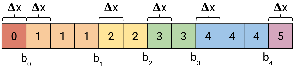
Figure 5: Array with indexes to the quantized activation function.
Memory savings?
Regular neural network models take a significant chunk of memory. It is caused by a large number of weights and their floating point representation (32 bits per weight). However, in the case of NMNF, we need to store only column indexes to the fixed size lookup table. For example, if we want to encode indexes to the lookup table with 1,000 unique weights, we can represent them with only 10 bits ($2^{9} < 1,000 < 2^{10}$) per weight, which can save up to 68.75 % memory compared to the floating point model. The NMNF paper does not mention it, but one of the current trends is to quantize weights to 8 bits [6]. Using 8 bit encoded weights yield 75 % memory savings with respect to floating point representation and 19.9 % memory reduction compared to NMNF representation.
Further, the authors claim that applying entropy coding to weights indexes can decrease the index size from 10 to 7 bits. We decided to put such a claim to the test (see Code 2). First, we sampled 60 million weights (same as a number of weights in AlexNet) from Laplacian distribution (see Figure 5a) and clustered them with Mini Batch K-Means algorithm to 1,000 bins. From Figure 5b you can see that the number of weights in bins follow the Laplacian distribution as well.
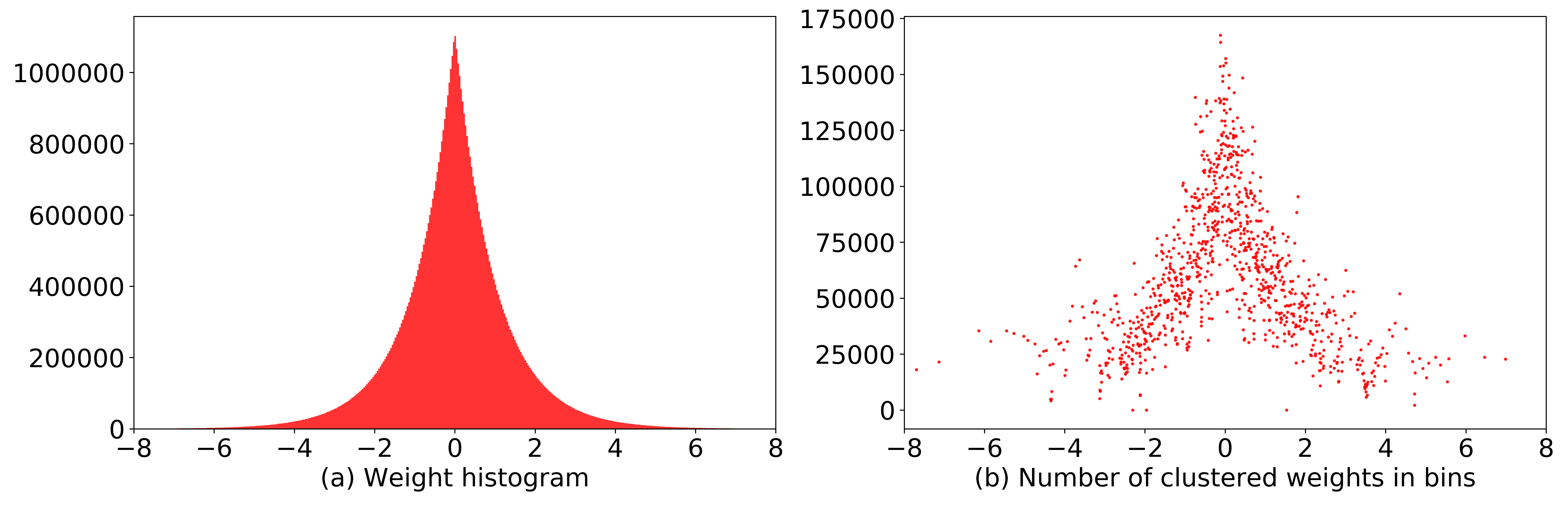
Figure 5: (a) Histogram of weights sampled from Laplacian distribution. (b) After the weight clustering step, the number of weights in bins keep the same data distribution as the original weights.
Finally, we computed the discrete probability distribution of clustered weight indices and information entropy. According to Shannon’s source coding theorem it is impossible to compress data such that the average number of bits per symbol would be less than information entropy of the data. Our calculated information entropy was 9.756 bits which signal that weight indexes cannot be encoded with less number of bits. Different weight indexes and clusters will yield different information entropy, but it is unlikely that 7 bits would be sufficient to encode them.
import numpy as np
import scipy as sc
from sklearn.cluster import MiniBatchKMeans

def information_entropy(data: np.array, base: int=2) -> float:
  """Calculate the entropy of a given data stream.
  """
  unique_elements, counts_elements = np.unique(data, return_counts=True)
  p_data = counts_elements / data.size
  return sc.stats.entropy(p_data, base=base)

num_weights = 60_000_000  # number of weights in AlexNet
num_unique_weigths = 1_000  # number of columns in lookup table

# Sample random weights
W = np.random.laplace(size=(num_weights, 1))

# Cluster weights
kmeans = MiniBatchKMeans(
    n_clusters=num_unique_weigths,
    init="k-means++",
    max_iter=100,
    batch_size=100,
    verbose=0,
    compute_labels=True,
    random_state=None,
    tol=0.0,
    max_no_improvement=10,
    init_size=3*num_unique_weigths,
    n_init=3,
    reassignment_ratio=0.01,
).fit(W)

# Assign weights to clusters
W_clustered = kmeans.predict(W)

# Compute information entropy
H = information_entropy(W_clustered, base=2)

print("Information entropy:", H)
Information entropy: 9.756370565749936
Code 2: Information entropy of 1,000 unique weights that follow Laplacian distribution is 9.756 bits. This entropy can change based on the number of weights in every bin.
No multiplication, no floating point in AlexNet
NMNF approach was evaluated on AlexNet network [1]. Modified AlexNet achieved comparable results with the floating point model utilizing ReLU6 activation function. The experiments have also shown that with quantized inputs the performance degradation is negligibly small.
| AlexNet | Recall@1 | Recall@5 |
|---|---|---|
| Floating point | 56.4 | 79.8 |
| NMNF floating point inputs | 57.1 | 79.8 |
| NMNF quantized inputs | 56.9 | 79.4 |
Table 2: Comparison of floating point and NMNF AlexNet model. NMNF model employed 1,000 unique weights and 32 quantized levels of ReLU6 activation function.
AlexNet contains one extra layer (dropout layer can be ignored during inference), max pooling, that has not been mentioned yet. Max pooling layers come after activation layers (see Figure 6). Fortunately, the order of quantized output values (row indexes of the lookup table) correspond to the order of their real values, thus max pooling in NMNF network can be performed without any modifications. On the other hand, if we had average pooling layer in our network we would have to convert indexes to their real values in order to compute average correctly. Also, similarly to our previously defined lookup table, we could precompute all possible averages and then match them with values in pooling windows.
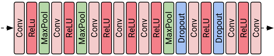
Figure 6: Visualization of AlexNet network.
Speed comparison
In the last part of our NMNF review, we will integrate convolution operation without multiplication into high-performance neural network inference computing framework called ncnn and discuss its consequences on inference time. We assume that NMNF network would be deployed on mobile devices with ARM-based processors since they cover about 95 % of market. The enabling technology behind fast execution of deep learning models on devices with ARM processors is ARM Neon, an advanced SIMD (single instruction multiple data) architecture extension for the Arm Cortex-A series and Cortex-R52 processors. Parallelism, highly optimized math functions and support for both float and 8-bit integer operations are a perfect fit for current deep learning models. For example, convolutional layers are composed of multiply & accumulate operations and this exact combination of operations can be executed using single instruction VMLA (Vector MuLtiply Accumulate). If we use both 8-bit weights and 8-bit activations, we can perform 16 multiply & accumulate operations in parallel. You can confirm that every major deep learning inference engine utilizes it.
int8x16_t vmlaq_s8(int8x16_t a, int8x16_t b, int8x16_t c); // VMLA.I8 q0,q0,q0
Code 3: vmlaq_s8 ARM Neon instruction can perform 16 multiplications of 8-bit integer and 16 addition of 8-bit integers in parallel using one instruction.
First, we measured inference time† of AlexNet floating point version using single big core on Galaxy Note 3 (see Figure 7) and Galaxy S8. Before the actual measurements were taken, 10 forward pass warm-up runs were executed. Following 10 runs were averaged to obtain the final layer-wise speed measurements. You can notice that the most time-consuming layer is the first convolutional layer and that convolutional layers take the most of the time overall (91.4 % for Galaxy Note 3 and 95.7 % for Galaxy S8). The reason that the first convolutional layer in AlexNet takes up so much time is its unoptimized implementation for kernels with uncommon sizes. For further measurements, we are not going to consider this layer (conv1) in our evaluation.
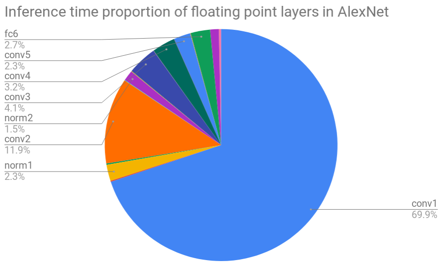
Figure 7: Layer-wise inference time breakdown of float AlexNet model run on Galaxy Note 3.
Next, we added NMNF convolution layers (3x3s1 and 5x5s1) supporting 32 activation levels and 1,000 unique weights. To facilitate correct execution of NMNF convolutional layers we swapped the position of convolutional layers and its succeeding activation layers. This modification ensures that there is always a limited number of unique activation values coming into NMNF convolutional layers. Since the swap would affect the speed measurements of activation layers, moreover, the most of the inference time is spent in convolutional layers, we continue to measure speed of convolutional layers only.
static void conv3x3s1_nmnf(
    const Mat& bottom_blob,
    Mat& top_blob,
    const Mat& _kernel,
    const Mat& _bias,
    const int lookup_table[NMNF_NUM_ACTIVATIONS][NMNF_NUM_WEIGHTS],
    const Option& opt
    )
{
    int w = bottom_blob.w;
    int h = bottom_blob.h;
    int inch = bottom_blob.c;

    int outw = top_blob.w;
    int outh = top_blob.h;
    int outch = top_blob.c;

    const int* kernel = _kernel;  // column index
    const int* bias = _bias; // column index to the last row of lookup table

    for (int p=0; p<outch; p++)
    {
        Mat out0 = top_blob.channel(p);

        const int bias0 = lookup_table[NMNF_NUM_ACTIVATIONS-1][bias[p]];
        out0.fill(bias0);

        const int* k = kernel + p*inch*9;
        const int* k0 = k;
        const int* k1 = k+3;
        const int* k2 = k+6;

        for (int q=0; q<inch; q++)
        {
            int* outptr0 = out0;
            int* outptr1 = outptr0 + outw;

            const int* img0 = bottom_blob.channel(q); // row index
            const int* r0 = img0;
            const int* r1 = img0 + w;
            const int* r2 = img0 + w*2;
            const int* r3 = img0 + w*3;

            int i = 0;

            for (; i+1 < outh; i+=2)
            {
                for (int ow=0; ow<outw; ow++)
                {
                    *outptr0 += lookup_table[r0[0]][k0[0]] + \
                                lookup_table[r0[1]][k0[1]] + \
                                lookup_table[r0[2]][k0[2]] + \
                                lookup_table[r1[0]][k1[0]] + \
                                lookup_table[r1[1]][k1[1]] + \
                                lookup_table[r1[2]][k1[2]] + \
                                lookup_table[r2[0]][k2[0]] + \
                                lookup_table[r2[1]][k2[1]] + \
                                lookup_table[r2[2]][k2[2]];

                    *outptr1 += lookup_table[r1[0]][k0[0]] + \
                                lookup_table[r1[1]][k0[1]] + \
                                lookup_table[r1[2]][k0[2]] + \
                                lookup_table[r2[0]][k1[0]] + \
                                lookup_table[r2[1]][k1[1]] + \
                                lookup_table[r2[2]][k1[2]] + \
                                lookup_table[r3[0]][k2[0]] + \
                                lookup_table[r3[1]][k2[1]] + \
                                lookup_table[r3[2]][k2[2]];

                    outptr0++;
                    outptr1++;

                    r0++;
                    r1++;
                    r2++;
                    r3++;
                }

                outptr0 += 2 + w;
                outptr1 += 2 + w;
            }

            // remaining
            for (; i < outh; i++)
            {
                for (int ow=0; ow<outw; ow++)
                {
                    *outptr0 += lookup_table[r0[0]][k0[0]] + \
                                lookup_table[r0[1]][k0[1]] + \
                                lookup_table[r0[2]][k0[2]] + \
                                lookup_table[r1[0]][k1[0]] + \
                                lookup_table[r1[1]][k1[1]] + \
                                lookup_table[r1[2]][k1[2]] + \
                                lookup_table[r2[0]][k2[0]] + \
                                lookup_table[r2[1]][k2[1]] + \
                                lookup_table[r2[2]][k2[2]];

                    outptr0++;

                    r0++;
                    r1++;
                    r2++;
                }

                outptr0 += 2;
            }

            k0 += 9;
            k1 += 9;
            k2 += 9;
        }
    }
}
Code 4: Implementation of 3x3s1 NMNF convolutional layer.
Figure 8 compares average speed of convolutional layers between our integrated NMNF and original floating point version from ncnn. NMNF convolutions are significantly slower than regular floating point convolutions for both tested devices. Surprisingly, the speed of floating point convolutions is very similar, even though Galaxy Note 3 is 4 years older than Galaxy S8. Slow execution of NMNF convolutional layers is a consequence of not utilizing ARM Neon parallel instructions. Albeit, there is VTBL instruction to perform fast parallel lookup search, the size of lookup table is limited to at most 4 registers which is considerably smaller than what we would need for or lookup table with 33,000 values. If we would like to use VTBL despite its limitations we would have to apply this instruction countless times (due to a large number of unique weights; column indexes) instead of the simple multiplication operation in order to obtain a correct result.
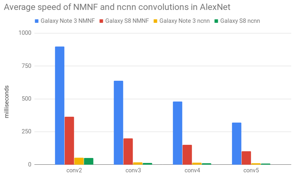
Figure 8: Average speed of NMNF and ncnn convolutions in AlexNet measured on Galaxy Note 3 and Galaxy S8.
In the NMNF paper they argue that their baseline implementation is 8 times faster than DoReFa-Net [7] although optimized implementation of DoReFa-Net has not been released. NMNF approach would benefit from small number of unique weights, which unfortunately leads to noticeably worse performance [1]. One of the main points is that relative speed of lookup versus multiplies empowers the NMNF network with great speed, but most likely this is only possible only with specialized architectures that support parallel search in large lookup tables.
Summary
No Multiplication? No floating point? No problem? Training networks for efficient inference proposes a new way of performing forward pass of the convolutional layer without using floating point multiplication operation. Weights and activations are quantized to the fixed number of values. Weights can be simply clustered with K-Means or model-based quantization approach. Activations are quantized uniformly in the output range. It is recommended to use 1,000 unique weights and 32 activation levels. During training, weights are quantized at predefined intervals and activations are quantized at every training step. Multiplication results of all quantized weights and activations form lookup table that is searched at inference time instead of computing product of weights and activations. Model weights are stored as indexes to lookup table and can be compressed to 10 bits per weight when using 1,000 unique weight values. Precomputed values in the lookup table can be converted to fixed point values without any negative effects. In the last part, we implemented NMNF convolutional layers and measured speed of NMNF AlexNet network with Samsung Galaxy Note 3 and Samsung Galaxy S8. Unfortunately, lookup table search operation has limited ways of parallelization therefore performs poorly on our benchmark compared to the regular floating point convolution. However, it is possible that custom hardware accelerator could perform significantly better if it supports parallelized search on a large lookup table.
Notes
† Benchmark application was executed via adb shell which can negatively affect time measurements.
They are caused by different behavior of Android’s scheduler between foreground Activity/Application and a regular background binary called from adb shell.
In this post, we evaluate the only relative speed of NMNF model versus floating point model, thus different scheduler behaviors should have no effect.
References
[1] S. Baluja, D. Marwood, M. Covell, N. Johnston: No Multiplication? No floating point? No problem? Training networks for efficient inference, 2018, link
[2] A. Anderson, A. Vasudevan, C. Keane, D. Gregg: Low-memory GEMM-based convolution algorithms for deep neural networks, 2017, link
[3] E. Vasilakis: An Instruction Level Energy Characterizationof ARM Processors, 2015, link
[4] A. Krizhevsky, I. Sutskever, G. E. Hinton: ImageNet Classification with Deep Convolutional Neural Networks, 2012, link
[5] D. Sculley: Web-Scale K-Means Clustering, 2010, link
[6] R. Krishnamoorthi: Quantizing deep convolutional networks for efficient inference: A whitepaper, 2018, link
[7] S. Zhou, Y. Wu, Z. Ni, X. Zhou, H. Wen, Y. Zou: DoReFa-Net: Training Low Bitwidth Convolutional Neural Networks with Low Bitwidth Gradients, 2018, link