Kill the bits and gain the speed?

Recently, Facebook AI Research in collaboration with University of Rennes released paper “And the Bit Goes Down: Revisiting the Quantization of Neural Networks” [1] which was accepted to ICLR 2020. The authors proposed a method of weight quantization for ResNet-like [2] architectures using Product Quantization [3]. Unlike many other papers, the error caused by codewords was not minimized directly. The training method aims to minimize the reconstruction error of fully-connected and convolutional layer activations using weighted $k$-means. Quantization was applied to all 3x3 and 1x1 kernel sizes except for the first convolutional layer. The paper emphasizes the importance of optimizing on in-domain input data in both quantizing and fine-tuning stages. Using their technique, weights in ResNet 50 can be compressed with a 20x factor while maintaining competitive accuracy (76.1 %). The potential impact of byte-aligned codebooks on efficient inference on CPU was briefly mentioned, but no actual method was presented. We propose and explore one possible way of exploiting frequent redundant codewords across input channels in order to accelerate inference on mobile devices.

The following post is divided into two parts: Method Overview, and Inference Acceleration.

Method Overview

We present an overview of methods used in a paper: Product Quantization, Codebook Generation and Network Quantization. For more details, we recommend reviewing the original paper [1].

Product Quantization

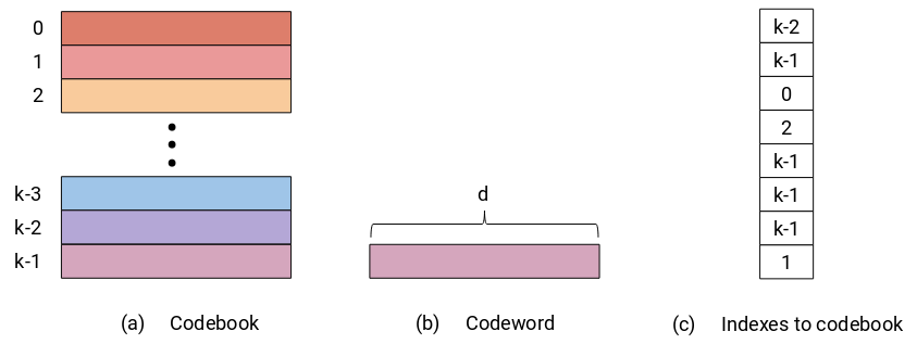
Product Quantization (PQ) is a general quantization technique that enables a joint quantization of arbitrary number ($d$) of components. The number of components is a hyperparameter, but as we can see later it can be chosen based on prior information about the data that we want to quantize. The dimensionality $d$ of quantized components does not change and neither does the data type precision. The main benefit of PQ comes from its compressed representation of quantized components defined by indexes pointing to a codebook. The codebook of dimensions $d \times k$ stores $k$ optimal centroids also called codewords. The number of codewords $k$ directly affects the size of a codebook and the data type that is used to store codeword indexes is defined by the number of codewords in the codebook (e.g. 1 Byte can hold up to 256 indexes). The codewords are derived from data, and the more frequent components can be quantized with a lower error. The quantization process itself is usually done using one of the clustering techniques, such as weighted $k$-means in the case of “And the Bit Goes Down”[1].

Codebook Generation

Product Quantization was utilized to quantize the weights of convolutional and fully-connected layers. The obvious objective of weight quantization is to minimize an error between original and quantized weights (Equation 1). This can seem like a valid approach, however, we should keep in mind that eventually, weights are just constants that are used to compute the actual activations. For this reason, an imprecise quantization does not manifest itself only in a weight error but also in a reconstruction error of the layer output. On the other hand, this objective requires to have access only to weights, and not the training data.

Equation 1: Objective function of quantization method for minimizing weight error.

The authors of the paper proposed an alternative objective function (Equation 2) that minimizes the reconstruction error. This objective function can be applied only during training to have access to input activations $x$. The training procedure is described in the following subsection.

Equation 2: Objective function of quantization method for minimizing reconstruction error.

The objective function from equation 2 can be minimized using weighted $k$-means in which weights are represented by input activations, and therefore the reconstruction error is scaled by the magnitude of input activations.

Until now, we have talked about layer weights and quantization in general but to fully exploit Product Quantization, layer weights should be split into coherent subvectors. This split is different for various layer types. Here, we describe the split for a fully-connected layer and later for a convolutional layer. The weight $W_{fc} \in R^{C_{in} \times C_{out}}$ of the fully-connected layer is first split into columns and every column is then further split into $m$ subvectors of size $d = C_{in} / m$, assuming that $C_{in}$ is divisible by $m$. Generated subvectors are utilized for quantization and the generation of codewords within the codebook.

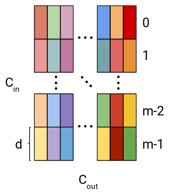
Figure 2: Visualization of weight split into subvectors in a fully-connected layer.

Convolutional weight $W_{conv} \in R^{C_{out} \times C_{in} \times K \times K}$ has an implicit spatial correlation between $K$’s dimensions where $K$ depicts the filter size. Using this knowledge, weight is reshaped into $W_{conv} \in R^{(C_{in} \times K \times K) \times C_{out}}$ and split along the first dimension into subvectors of size $K^2$ (e.g. subvectors of size 9 for 3x3 convolution).

Network Quantization

Network quantization starts from a pre-trained network and in its first phase layers are quantized and finetuned independently in a sequential manner, from the lowest ones up to the final output layer. Input activations $x_{i}$ in layer $L_{i}$ are used in the process to quantize weights $W_{i}$ and according to [1], 100 finetuning steps for every layer are sufficient to converge. During finetuning, the quantized network is optimized using KL loss between the output of the quantized network and output from floating-point teacher network [4] of the same architecture.

After all layers are quantized and locally finetuned, global finetuning, the second phase of network quantization, can start. The global finetuning phase trains all codebooks jointly and additionally, a running mean and variance of Batch Normalization layers [5] are updated as well.

Inference Acceleration

“And the Bit Goes Down” [1] achieves good compression ratios, using PQ and half-precision floating-point weights, however, the paper does not go beyond the compression use case. Network compression is usually just one necessary ingredient for deploying trained networks on edge devices. With smaller networks we can save the bandwidth while transmitting the latest model to the remote device, and also save the space in a local memory of a device, however, the memory footprint and inference time are no less important for edge devices. In this section, we will describe one possible acceleration technique for the convolutional layer in the PQ network and evaluate it on a mobile device.

Acceleration Proposal

One famous technique that compresses the size of a network and implicitly accelerates its inference time is channel pruning [6]. Channel pruning removes whole channels from the given weight, which results in less computation in the current layer and also in the previous one.

Weights in PQ network have the same shape as those in an original non-quantized network, therefore we cannot achieve similar speedups as with channel pruning technique, however, we can exploit the fact that every layer has limited number of unique codewords and that some of those codewords can repeat within the same group of input channels. In the figure below, we conceptualize repeated codewords within the same group of input channels using colors (every column has at least two identical codewords).

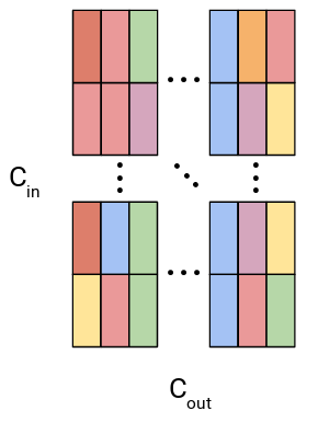
Figure 3: Visualization of weight split into subvectors in a fully-connected layer with repeated codewords within the same group of input channels.

Convolution is composed of two operations: multiplication and addition, and for single output value can be defined as follows:

where $x_i$ represents single value input activation, $w_i$ is a single value from weight $W$, and $K^2$ defines weight size. Convolution satisfies distributive property which we will use to decrease the number of multiplication operations. In the following equation, we demonstrate how the optimized convolution would work. Notice that the red color weight $\color{red}{w_0}$ repeats three times. This allows us to first sum up activations that were paired with $\color{red}{w_0}$ and only after that we multiply $\color{red}{w_0}$ with summed activations. With this approach, a number of saved multiplication operations is proportional to number of repeated weight values.

This method can be readily applied to PQ networks because with a limited number of unique codewords we can expect a codeword redundancy within the same group of input channels. In the next section, we describe how we implemented and evaluated the proposed acceleration technique for ResNet 18 network.

Analysis & Implementation

The authors released an implementation of paper together with several pre-trained models. For our analysis, we use ResNet 18 network as an example and all experiments are measured on One Plus 6t and Samsung Galaxy Note 3 running modified ncnn inference engine.

Theoretical Speedup

The computational cost of standard convolution is defined as

where $K \times K$ represents kernel size, $M$ number of input channels, $N$ number of output channels, and $D_x \times D_x$ size of input activation. Proposed acceleration can be viewed as a preprocessing step of input activations before they are fed into a convolution operation. Such preprocessing would channel-wise sum up input activations that share the same weight codewords and as a result number of input channels would decrease.

To be able to compute a theoretical speedup of proposed acceleration we must have access to the codebook for every layer. Fortunately, the pre-trained ResNet 18 model contains such codeword indexes. From this information, we can obtain a number of unique codewords that would be used for the computation of a single output channel. The number of unique codewords varies between output channels, however, to simplify the computation of the theoretical speedup, we decided to make use of the maximum number of unique codewords across all output channels for every layer. With this, we obtain a minimal theoretical speedup reaching almost 20 % of computational cost. In the figure below, you can see that the reduction of input channels is more pronounced in the latter parts of the network, where the original number of input channels stretches up to 512.

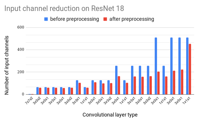
Figure 4: Number of input channels before and after preprocessing of input activations for every convolutional layer.

Layer-wise Analysis

To put a theoretical speedup into perspective, we measured an inference time of floating-point ResNet 18 network. The execution of all layers took about 187 ms and 299 ms on One Plus 6t and Samsung Galaxy Note 3, respectively. From the figure below, we can see that most of the time (89.2 % for One Plus 6t) is spent in 3x3 convolutions and the second most time-consuming layer is 7x7 convolution. Our focus is only on 3x3 convolution because 7x7 convolution is part of the first layer which was not quantized.

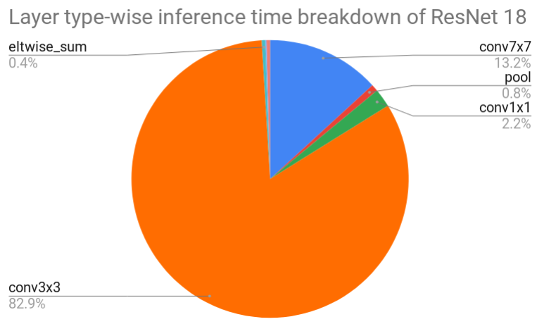
Figure 5: Layer type-wise inference time breakdown of floating-point Resnet 18 network executed on One Plus 6t.

Many 3x3 convolutional layers cost around 11 ms (One Plus 6t). The most frequent input activation shapes are 56x56, 28x28, 14x14 and 7x7 with 64, 128, 256 and 512 input channels, respectively. Later, we will benchmark these convolutions to find out the actual computational speedup.

Implementation

To be able to verify the theoretical speedup, we modified ncnn inference engine and integrated our proposed inference acceleration method. We added a channel-wise summation of input activations with a randomly generated codeword assignments limited by the number of unique weight codewords per input channel. The summation was implemented using NEON intrinsics to exploit parallel processing capabilities of the ARM processor and the memory used to store the summed up input activations were allocated in advance, during the network initialization. Convolutional weights need to be altered in a way that acknowledges changes within input activations, specifically by shifting and removing weight codewords. In our implementation, however, we allocate only weights of correct shape, without correct weight initialization. While this implementation promises an accelerated inference time, it should be noted that it has a larger memory footprint due to the extra preallocated input activations and weights.

Benchmarking Optimized Convolution

In the following figures, we compare the inference time of original 3x3 convolution (denoted as w/o reduction) with 3x3 convolution enhanced by preprocessing of input activations (denoted as w/ reduction).

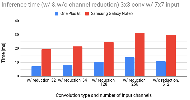
Figure 6: Comparison of 3x3 convolution with and without channel reduction for 7x7 input.

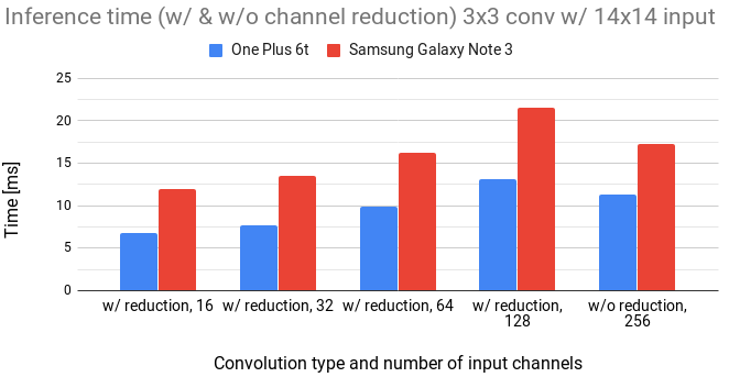
Figure 7: Comparison of 3x3 convolution with and without channel reduction for 14x14 input.

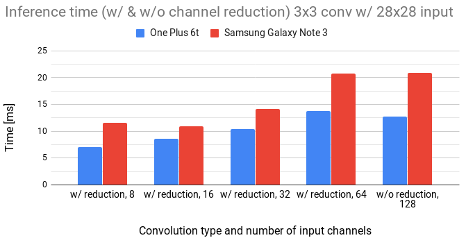
Figure 8: Comparison of 3x3 convolution with and without channel reduction for 28x28 input.

We notice that the inference time linearly increases with the number of input channels. We can also see that to gain any speed, the number of channels has to be reduced approximately by a 4x factor. The overhead in channel reduction seems to be quite high. It is caused by access to every channel of input activation and channel-wise summation operation. Moreover, the implementation of the convolutional layer exploits vmla SIMD instruction that can multiply and accumulate four single-precision floating-point values in parallel using only one instruction.

float32x4_t vmlaq_f32(float32x4_t a, float32x4_t b, float32x4_t c);

Code 1: vmlaq_f32 ARM Neon instruction can perform 4 multiplications of 32-bit floating-point and 4 additions of 32-bit floating-point in parallel using one instruction.

As a result, the summation in the convolutional layer is used for free. Our method, therefore, does not move it out of convolution as it might seem from equation 2 but introduces extra new summation operations. Unfortunately, with the current pre-trained PQ ResNet 18 network, where the largest channel compression per layer is slightly above 50 %, we wouldn’t be able to accelerate the inference, unless the number unique codewords for every channel gets smaller.

Summary

“And the Bit Goes Down: Revisiting the Quantization of Neural Networks” [1] proposes a quantization technique that combines a Product Quantization with careful layer-wise pretraining and local/global finetuning using fixed teacher network. Network weights are quantized using weighted $k$-means with an objective function that tries to minimize a reconstruction error, instead of minimizing weight error directly. The proposed method achieves high compression rates on Resnet-like architectures, however, there was no suggestion in the paper how we could accelerate an inference time with such a quantization scheme.

We proposed a method that modifies input activations and convolutional weights to reduce the number of multiplications in a convolutional layer. By benchmarking on a One Plus 6t and a Samsung Galaxy Note 3, we confirmed a speedup of convolution using our method. However, in order to achieve any meaningful speed gains the number of channels has to be reduced by at least a factor of 4x.

Notes

All experiments were launched using a modified ncnn benchmark on a One Plus 6t with Snapdragon 845 and a Samsung Galaxy Note 3 with Snapdragon 800. Every measurement was obtained by averaging 200 continuous runs and removing outliers from the first and last quartile of inference duration distribution. Lastly, we always used only a single big core, since it reflects the best an allowed computational power in real-world scenarios.

References

[1] P. Stock, A. Joulin, R. Gribonval, B. Graham, H. Jégou: And the Bit Goes Down: Revisiting the Quantization of Neural Networks, 2019, link
[2] K. He, X. Zhang, S. Ren, J. Sun: Deep Residual Learning for Image Recognition, 2015, link
[3] H. Jegou, M. Douze, C. Schmid: Product Quantization for Nearest Neighbor Search, 2011, link
[4] G. Hinton, O. Vinyals, J. Dean: Distilling the Knowledge in a Neural Network, 2015, link
[5] S. Ioffe, C. Szegedy: Batch Normalization: Accelerating Deep Network Training by Reducing Internal Covariate Shift, 2015, link
[6] Y. He, X. Zhang, J. Sun: Channel Pruning for Accelerating Very Deep Neural Networks, 2017, link